Monitoring & Targeting
A clear operator view, supported by the data, calculations and evidence behind every dial.
Start here
Read the dashboard in this order
| Section | The operator's question | ||
|---|---|---|---|
| 1 | Monthly Energy Target | How much of the monthly allowance have we used, and will we stay within it? | OPEN |
| 2 | Power Factor | How effectively are we using the available electrical capacity? | OPEN |
| 3 | kWh per ton | How much energy does each ton require, and what should it require? | OPEN |
| 4 | Predicted Demand | Where will this demand interval finish against the 4.5 MVA limit? | OPEN |
| 5 | Plant Efficiency | Are we using more or less energy than the baseline expects? | OPEN |
Explore supporting views:
- Baseline scatter
- Running empty
- Service-output baselines
- Demand control
- Savings & M&V
- Energy balance
- Action and integration
- Technical notes
The dashboard is the front end of the same measurement system: measure, compare with expected performance, act and verify.
Dial 1 · Monthly Energy Target
What is the monthly energy target?
The operator’s question: How much of the monthly allowance have we used, and will we stay within it?
The monthly energy target is the approved kWh allowance for the production and operating conditions planned for the month. The dial shows how much has been used and how much remains. Its supporting forecast shows whether month-end energy is likely to exceed the allowance.
Read the dial with its forecast
- Used: month-to-date metered energy as a percentage of the approved monthly target.
- Remaining: the target less actual energy already consumed. A negative balance means the allowance has been exceeded.
- Forecast: actual energy to date plus the energy expected for the remaining production plan.
Used (%) = actual month-to-date kWh ÷ monthly target kWh × 100
Forecast month-end kWh = actual to date + expected remaining kWh
Worked example: 72% used does not tell the whole story
| Measure | Illustrative value |
|---|---|
| Approved monthly target | 1,000,000 kWh |
| Actual energy used to date | 720,000 kWh = 72% used |
| Allowance remaining | 280,000 kWh = 28% remaining |
| Energy expected for remaining production | 300,000 kWh |
| Forecast month-end energy | 1,020,000 kWh |
| Forecast excess | 20,000 kWh, or 2% above the allowance OVER |
Set the target from the production plan
Apply the approved baseline model to planned output and operating periods, then include any separately agreed improvement target. Compare actual use with the expected trajectory for actual production, rather than elapsed calendar days alone.
If the production plan, product mix or operating boundary changes, record and approve the adjustment. Do not increase the target simply to absorb inefficient operation. Baseline expectation and a tighter improvement target must be clearly distinguished.
Operator response
If the forecast is above target, open the interval exceptions and baseline scatter. Identify running empty, unstable loading or persistent excess use; assign actions before the remaining allowance is consumed.
Read the energy balance together with the production forecast. "72% used" alone is not an efficiency judgement.
Dial 2 · Power Factor
What is power factor?
The operator’s question: How effectively are we using the available electrical capacity?
Power factor (PF) is the ratio of real power, which performs useful electrical work, to apparent power, which determines the loading on the electrical supply. For a normal importing load, a value closer to 1.00 means less apparent power is required for the same real power.[1]
Power factor = real power (kW) ÷ apparent power (kVA)
Use the meter's true power-factor value. In a system with waveform distortion, power factor is not simply the cosine of the phase angle. PF is an electrical-capacity indicator; it is not the same as production efficiency or kWh per ton.
Read the dashboard example
| Indication | Meaning |
|---|---|
| Live PF: 0.97 | The example is above the proposed 0.95 target. |
| GREEN 0.95–1.00 | Within the proposed preferred range. |
| AMBER 0.80 TO BELOW 0.95 | Investigate correction and loading. |
| RED BELOW 0.80 | Escalate against the agreed site alarm rules. |
Confirm before commissioningThese colour bands are design settings, not universal tariff thresholds. Confirm the site's requirements, importing/exporting sign convention and leading/lagging indication before commissioning.
Worked example: the same 1,000 kW load
| Power factor | Apparent demand |
|---|---|
| 0.80 | 1,000 ÷ 0.80 = 1,250 kVA |
| 0.95 | 1,000 ÷ 0.95 = 1,052.6 kVA |
| Difference | About 197.4 kVA less apparent demand |
The reduction in kVA can release capacity and affect demand charges, subject to the tariff. It is not an equivalent reduction in kWh: real energy and electrical losses must be assessed separately.
Operator response
Check whether poor PF coincides with lightly loaded equipment, a failed correction stage or a change in plant operation. Refer correction settings, harmonics and the risk of leading PF or overcorrection to the responsible engineer.
PF explains electrical loading. The next dial explains energy used for useful production.
Dial 3 · Specific Energy
What does kWh per ton mean?
The operator’s question: How much energy does each ton require, and what should it require?
Specific energy, expressed as kWh/t, is the electrical energy used to produce one ton of output. The numerator and denominator must cover the same plant boundary and the same time interval. This document uses metric tonnes (t); the dashboard label "TONS" must use the same convention.
Specific energy (kWh/t) = interval energy (kWh) ÷ interval output (t)
Worked example: compare actual with expected
| Measure | Same interval (example) |
|---|---|
| Actual energy and output | 8,200 kWh and 1,000 t |
| Actual specific energy | 8,200 ÷ 1,000 = 8.2 kWh/t |
| Baseline energy at that output | 7,200 kWh, equivalent to 7.2 kWh/t |
| Excess above baseline | 1,000 kWh, or 1.0 kWh/t |
How the baseline provides the target
A simple production model may take the form below. The fixed term represents energy that does not vary directly with output within the modelled operating state; the variable term describes the additional energy associated with production.
Expected interval energy = fixed term + variable rate × tonnes
For example, an illustrative model of 2,200 + 5.0 × tonnes predicts 7,200 kWh at 1,000 t. The expected kWh/t is therefore 7.2 at that output. At a different output, the expected ratio changes because the fixed term is spread over a different number of tonnes.
Data rules for a trustworthy dial
- Match timestamps and intervals. Instantaneous MW and cumulative tonnes cannot directly produce interval kWh/t.
- For a shift or month, divide total energy by total tonnes; do not take an unweighted average of interval ratios.
- At zero or very low output, show an idle or running-empty flag. Do not divide by zero or show a misleading zero kWh/t.
- Display the interval, data status and baseline version. Confirm the illustrative 0–12 scale and target bands from site data.
kWh/t is meaningful only when output, operating conditions and the expected baseline are understood together.
Dial 3 continued · Building the baseline
Use the scatter to explain kWh/t
Each point pairs energy and production from one interval. A validated model describes expected energy across the operating range. The scatter shows where performance departs from that expectation and where further investigation is needed.
Create the baseline in four steps
- Collect representative, time-aligned energy, production and operating-state records. Cover the normal production range and relevant seasonal or product-mix effects.
- Check missing values, meter resets, shutdowns and abnormal states. Retain an audit trail of exclusions; separate different operating modes where required.
- Fit an appropriate model and examine residuals, bias and validity range. A visually neat line or a high correlation alone is not sufficient validation.
- Approve the baseline, its uncertainty/tolerance and adjustment rules before using it for the live dial or savings verification.[4]
Read the points
Above the baseline: more energy than expected for the same output. Near or below it: potentially normal or improved performance, subject to data checks. At little or no output: investigate running empty separately, even if the points lie below the productive-operation baseline.
The annotated examples show 7,900 kWh ÷ 500 t = 15.8 kWh/t, compared with 8,200 kWh ÷ 1,000 t = 8.2 kWh/t. Specific energy is about 48% lower at the higher output; this demonstrates a loading effect, not verified savings from an intervention.
Dial 3 continued · Running empty
Separate idle use from productive use
The supplied historical scatter makes running empty visible: the cluster at zero production shows substantial electrical input while no useful output is recorded. This is a priority for scheduling and operating-state investigation.
Read the source units correctly
- The source plots kW against tonnes with a stated ×4 display scaling. It is a power-versus-production graph, not the kWh-versus-tonnes graph on the previous page.
- Under that convention, divide the plotted horizontal value by four to recover tonnes. Confirm the interval, original units and scaling with the source data before use.
- The red line is the supplied operating reference. Validate its derivation before treating it as an approved regression baseline.
Energy associated with a power difference = kW difference × duration (hours)
Confirm from source recordsA vertical gap on this graph is in kW. Convert it to kWh using the relevant duration, then judge how much is avoidable. The title's "26% of the time" is a historical source statement; confirm it from timestamps and operating-state records, not the appearance of the scatter alone.
Use running-empty periods to review shutdown discipline, interlocks and sequencing, while preserving essential services and safe process conditions.
Dial 3 continued · Service-output baselines
Compare at the same useful output
Not every plant produces tonnes. Compressors, pumps and other utilities use the same baseline principle with an appropriate service measure, such as delivered air volume or water pumped. Compare equivalent service and operating conditions.
What the lower curve means
At comparable airflow, a lower kW curve indicates less electrical input for the same service, provided pressure, air quality and other material conditions are equivalent. Integrate the difference over operating time to estimate the associated kWh reduction.
The historical example reports an average reduction of 138 kW (37%). Retain this as a reported result until the original validated data and calculation are available; do not use it as a guaranteed site saving.
Use the comparison to direct work
- Check unloaded running, leaks, setpoints, sequencing and operation away from the efficient service range.
- Compare baseline and post-action performance at equivalent airflow and pressure, with documented adjustments where conditions changed.
- Choose a consistent energy-per-service unit for the detailed view. Do not substitute instantaneous kW per flow unit for a measured energy-per-volume result without matching the time basis.
Whether the useful output is tonnes, air or water, the question is the same: how much energy should this service require?
Dial 4 · Predicted Demand
What is predicted demand?
The operator’s question: Where will this demand interval finish against the 4.5 MVA limit?
Predicted demand estimates the average demand that will be recorded when the current demand period closes. It gives the operator time to respond before the final interval value is established. The dashboard compares the prediction with the notified maximum demand (NMD) limit of 4.5 MVA.
Keep three quantities distinct
| Quantity | What it means |
|---|---|
| Live load | The present kW or kVA reading; it can change rapidly. |
| Completed interval demand | The average over the configured demand period. This document illustrates fixed 30-minute blocks. |
| NMD limit: 4.5 MVA | The agreed supply limit used for comparison; it is not the measured monthly peak. |
Why the interval matters
A high completed demand interval can set a monthly maximum. The amount billed depends on the site's tariff: eligible periods, kW or kVA basis, minimum demand, ratchets and NMD provisions must all be confirmed. A brief instantaneous peak is not automatically equal to a high 30-minute average.
Read the forecast and time remaining together. A 3.9 MVA prediction is an estimate of the closing interval, not a fixed allowance to add load.
Dial 4 continued · Calculation and response
How is demand predicted?
A simple fixed-block forecast adds the demand accumulated so far to the demand expected over the remaining time, assuming the recent load continues. Divide that total by the full block duration.[2]
Predicted kVA = (accumulated kVAh + recent kVA × hours remaining) ÷ block hours
Example: 12:45 remains in a 30-minute block. That is 0.2125 hours remaining and 17:15 elapsed. The accumulated value is 1,100 kVAh; recent load is 4,000 kVA.
| Calculation | Result |
|---|---|
| Expected addition | 4,000 × 0.2125 = 850 kVAh |
| Predicted closing demand | (1,100 + 850) ÷ 0.5 = 3,900 kVA = 3.9 MVA |
| Margin to 4.5 MVA limit | 4.5 − 3.9 = 0.6 MVA (600 kVA) WITHIN |
Illustrative forecastThis is an illustrative forecast, not a guarantee. Recalculate as load changes and retain an operating margin. Use the meter's approved demand method and clock alignment; some tariffs derive kVA from demand kW and kvar rather than a direct kVAh average.
Respond before the interval closes
Warn early, then shift, shed or sequence approved non-critical loads. Protect critical processes; use agreed deadbands, minimum run times and a controlled restoration sequence.
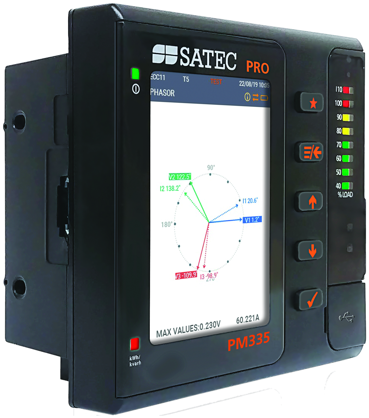
Meter implementation noteSATEC PRO distinguishes accumulated block demand from predicted sliding-window demand. The example above explains a fixed block; confirm the actual register, interval and controller algorithm against the billing method before commissioning.[3]
Dial 5 · Plant Efficiency
Derive efficiency from the baseline
The operator’s question: Are we using more or less energy than the baseline expects?
The Plant Efficiency dial summarises whether the plant used more or less energy than expected for the output achieved. Here, "efficiency" is an energy-performance index against the approved baseline, not a thermodynamic conversion efficiency.
Baseline performance index (%) = actual kWh ÷ expected baseline kWh × 100
For the same interval, the same positive output and the same boundary, this is also actual kWh/t divided by expected kWh/t, multiplied by 100. The kWh/t dial provides the specific value; Plant Efficiency summarises its position against the baseline.
Worked example from the centre dial
| Step | Calculation |
|---|---|
| Actual specific energy | 8.2 kWh/t |
| Expected baseline specific energy | 7.2 kWh/t |
| Performance index | 8.2 ÷ 7.2 × 100 = 113.9% HIGH / OFF TARGET |
| Energy above baseline | 13.9% |
| Excess at 1,000 t | (8.2 − 7.2) × 1,000 = 1,000 kWh |
Translate the index into a clear status
| Status | Interpretation |
|---|---|
| BELOW TARGET | Less energy than expected. Validate the data and operating conditions before accepting improvement. |
| ON TARGET | Within the approved tolerance around 100%. Set tolerance from model uncertainty and operational needs. |
| HIGH / OFF TARGET | Above the approved upper tolerance. Open the baseline scatter and interval exceptions. |
| IDLE / DATA UNAVAILABLE | No valid comparison because output, energy or baseline information is missing or unsuitable. |
If 8.2 and 7.2 kWh/t refer to the same interval and baseline, the live index is 113.9%: above baseline, not 100%.
Configure from the approved indexThe opening dashboard's 113.9% HIGH / OFF TARGET indication follows the illustrative 8.2 and 7.2 kWh/t values. During the live build, calculate the status from the approved index and tolerance; do not set it independently. Keep a tighter improvement target distinct from the baseline. Missing data must never default to a green status.
The link back to action
Use the same production, operating-state and baseline records for both dials. An adverse index leads back to its cause: running empty, part loading, process changes or equipment condition. Confirm the cause before assigning corrective work.
From dashboard to results · Measurement & Verification
Convert variance into verified savings
The dashboard points to a problem; the baseline quantifies the energy difference. A positive variance is an investigation opportunity, not proof that every excess kWh is avoidable. Savings are verified after action against an appropriately adjusted baseline.[4]
Illustrative interval calculation
| Measure | Value |
|---|---|
| Actual interval energy | 8,600 kWh |
| Baseline expected energy | 7,800 kWh |
| Positive energy variance | 800 kWh |
| Illustrative energy tariff | R1.80/kWh |
| Potential energy-cost opportunity | 800 × R1.80 = R1,440 |
Verify the result after the action
- Record the intervention, date, boundary and expected effect. Agree the comparison period and any baseline adjustments.
- Compare measured post-action energy with baseline energy predicted for the same output and relevant conditions. Check missing data and changed operating states.
- Report validated kWh savings, the applicable energy cost and any separately calculated demand-cost effect. Retain the model version and evidence.
Use the same data stream to identify the opportunity and verify the result. Do not count a kVA reduction as an equivalent kWh saving.
Supporting measurement · Energy balance & data
See where the energy is going
Meters at the incoming supply, major plants and utilities create a reconciled energy balance. It identifies the largest users and directs plant-level investigation. Reconcile the same period and explain unmetered use, losses and differences in meter boundaries.
Build one trusted data foundation
| Source | What it contributes |
|---|---|
| Electrical meters / ExpertPower | kWh, kW, kVA, PF, demand registers and load profiles. |
| SCADA and plant PLCs | Operating state, process conditions, equipment status and control response. |
| Production or service records | Tonnes, air or water volumes, or units over the matching interval. |
| Tariffs and approved targets | Energy rates, demand rules, NMD limit, monthly allowance and performance bands. |
| Baseline register | Boundary, valid range, exclusions, version, approvals and adjustment history. |
Keep the engineering detail behind the simple operator view. Every dial must support drill-down to the source trend, scatter, interval record and data-quality flags that created its indication.
Operating response · Action & integration
Turn the indication into a response
Monitoring & Targeting connects the symptom to its operating cause. Assign an owner and a due date, record what changed, then return to the same baseline to check the result.
| Opportunity | Data signal | Typical response |
|---|---|---|
| Above-baseline energy | Actual kWh exceeds expectation at the same output. | Check control loops, process settings, equipment condition and maintenance. |
| Running empty | Material energy use at little or no productive output. | Review scheduling, shutdown discipline, interlocks and stop/start sequencing. |
| Part loading | High kWh/t at low or unstable throughput. | Consolidate production and sequence equipment closer to its efficient range. |
| Maximum demand | Forecast approaches the configured limit. | Shift or sequence approved discretionary loads; protect critical processes. |
| Low PF / power quality | Poor PF, high kVA or power-quality events. | Review correction, harmonics and equipment loading with the engineer. |
| Pumps and utilities | Drift from the service-output baseline. | Check the operating point, controls and maintenance requirements. |
Commission the live dashboard carefully
- Match timestamps, meter boundaries, output units and intervals. Publish a visible timestamp and data-status flag; mark stale values clearly.
- Approve the model, validity range and adjustments. Set kWh/t bands and efficiency tolerance from the same baseline and operating period.
- Confirm PF bands, the 4.5 MVA NMD limit, demand-window settings, billing alignment and the monthly production-based allowance.
- Test calculations and alarm transitions with recorded scenarios: normal operation, no output, missing data, peak demand and changed production.
- Start with passive visibility. Add approved automatic actions only after controls, safety priorities, fallbacks and restoration logic have been tested.
Keep the display clear
Use circular dials without stretching, smaller outside dials, very light grey faces and crisp, solid colour bands. Retain centred centre-dial readouts and the complete red label "MAX DEMAND LIMIT 4.5 MVA". Pair colours with words and values so the status remains understandable without colour alone.
Measure continuously, integrate safely and verify every improvement against the agreed baseline.
Supporting views · Technical notes
Keep the evidence behind every dial
The opening dashboard supports immediate decisions. The following views retain the engineering detail and the audit trail needed to explain each indication.
| View | Purpose |
|---|---|
| Overview | Five dials, current alarms, operating status and action prompts. |
| Energy Balance | Incoming supply reconciled to plants, utilities and major feeders. |
| Baseline Scatter | Energy versus output, approved model, tolerance and interval detail. |
| Interval Exceptions | Above-baseline, running-empty and part-load periods ranked by energy, cost and recurrence. |
| Load Profile & NMD | Current demand period, prediction, monthly peak and controllable loads. |
| Power Factor & PQ | PF trend, kVA impact, power-quality events and affected feeders. |
| Savings & M&V | Adjusted baseline versus actual, verified savings and audit trail. |
| Data Quality & Baseline Register | Mapping, missing data, time alignment, exclusions, validity and approval history. |
| Action Tracker | Owner, due date, status, expected benefit and verified result. |
Technical references
- [1]SATEC — Power Meters: Power Factor. Real and apparent power definitions.
- [2]SATEC — Power Meters: Predicted Demand. Forecast principle using accumulated energy and present load.
- [3]SATEC — EM235/PM335 PRO Installation and Operation Manual, Rev. A8, pp. 62–63. Accumulated block and predicted sliding-window demand; verify installed settings and firmware.
- [4]US Department of Energy FEMP — Measurement and Verification Activities. Baseline conditions, M&V planning and documented adjustments.
Publication and configuration status
Before web publicationThis document combines the approved dashboard design, the supplied running-empty graph and the existing Monitoring & Targeting illustrations. The examples do not represent one common site dataset. Before web publication, confirm historical chart labels, units, dates and reported savings. Configure live values, targets, tolerances and tariff logic from approved site records.
Management sees where energy is used, engineers can explain the baseline, and operators can act on performance with access to the evidence.